When working with data imports in RandomPicker.com, you need to adhere to a specific Excel file format:
- Column 1: entry name (mandatory)
- Column 2: internal note (optional)
- Column 3: weight (optional)
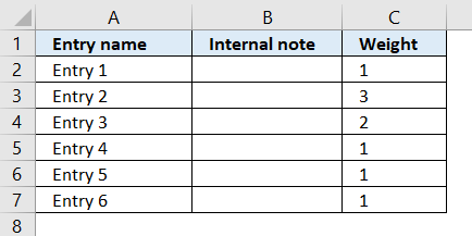
As you can see, the whole entry name must be placed in the first column of the spreadsheet. In some situations, you have multiple parts of the entry name in different columns (customer ID, first name, last name, city, etc.) so you need to merge the cells into one cell in each row. In this article, we will guide you through the process of concatenating cells in Excel.
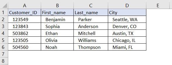
Step 1: Identify the columns to concatenate
First, determine which columns contain the information you want to merge. For instance, if you have separate columns for customer ID, first name, last name, and city, note their column headers and locations.
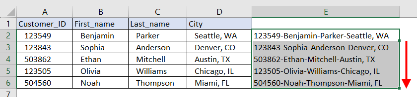
In our example, there are four columns to be merged: A,B,C,D.
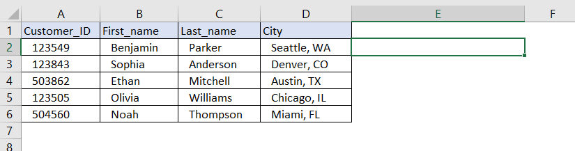
Step 2: Combine the cells using concatenate formula
Go to the cell where you want to merge the data. Let’s assume this cell is E2 (E2 means column E, row number 2) in the spreadsheet grid.
Then, enter the following formula into the formula bar:
=CONCATENATE(A2 & “-” & B2 & “-” & C2 & “-” & D2)
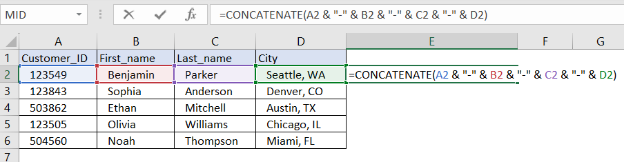
In this example, A2 represents the cell in the Customer_ID column, B2 represents the cell in the first name column, C2 represents the cell in the last name column, and D2 represents the cell in the city column. In this formula, we’ve used a hyphen (-) as the separator between the merged values. You can replace the hyphen with any other character or string that suits your needs, such as a comma, semicolon, or any other symbol. You can also add spaces or any additional text between the quotes. Hit the Enter key and you should see the merged text in E2.
Step 3: Copy the formula down
Once you have entered the formula in the first row, click on the bottom right corner of the cell and drag it down to apply the formula to the remaining rows in the column. Excel will automatically adjust the cell references for each row.
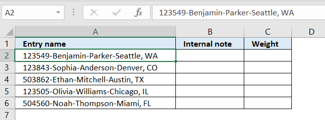
Step 5: Copy the merged data into a new spreadsheet as values
Once you have concatenated the desired data into a single column, copy it into a new spreadsheet as values. This ensures that the merged data remains intact and independent of the original spreadsheet. Follow these steps:
- Select the entire column E containing the merged data.
- Right-click on the selected column and choose “Copy” from the context menu, or use the shortcut Ctrl+C.
- Open a new Excel spreadsheet.
- Right-click on the cell where you want to paste the merged data and choose “Paste Values” from the context menu.
The merged data will be pasted into the new spreadsheet as values only, without any formulas or references to the original data.
You can also add the other two columns for the RandomPicker import – Internal note and Weight. They are optional, so you can proceed only with the Entry name column, too.
By following these simple steps, you can easily concatenate several columns in Excel into one cell. This technique is when you need to merge participant information for a raffle or any other data that is spread across multiple columns. Utilizing the CONCATENATE formula and the flexibility of Excel, you can combine and organize your data, saving time and improving your overall workflow.
Remember to always save a backup of your data before performing any modifications to ensure you can revert to the original state if needed.